Weather Typing for Climate Extremes
CEVE 543 - Fall 2025
2025-10-29
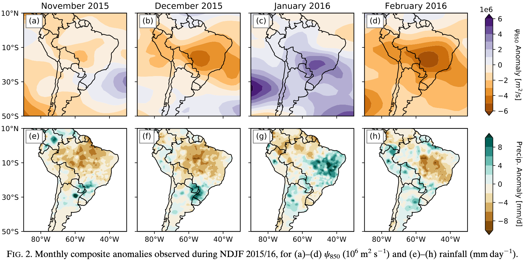
Q1: What was the large-scale climate picture during this period?
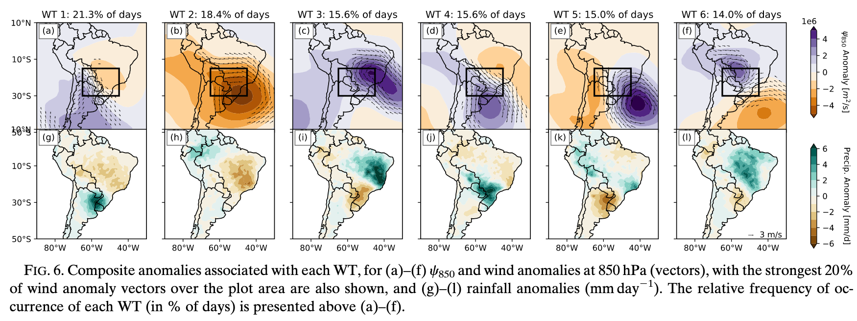
Q2: The authors explain this flood event through specific weather patterns called Weather Types (WTs). Looking at Fig. 6, what two fields are shown for each of the 6 weather types? Why are these appropriate choices?
Q3: Pick WT1 from Fig. 6 and describe it. What kind of circulation pattern does it show? Where does it rain? Where is the moisture coming from?
Q4: Now contrast WT1 with WT4 in Fig. 6. How do these two patterns differ in terms of circulation, precipitation, and moisture transport?
Q5: Which weather type(s) in Fig. 6 would you expect to be associated with heavy rainfall in the Lower Paraguay River Basin? What about dry conditions?
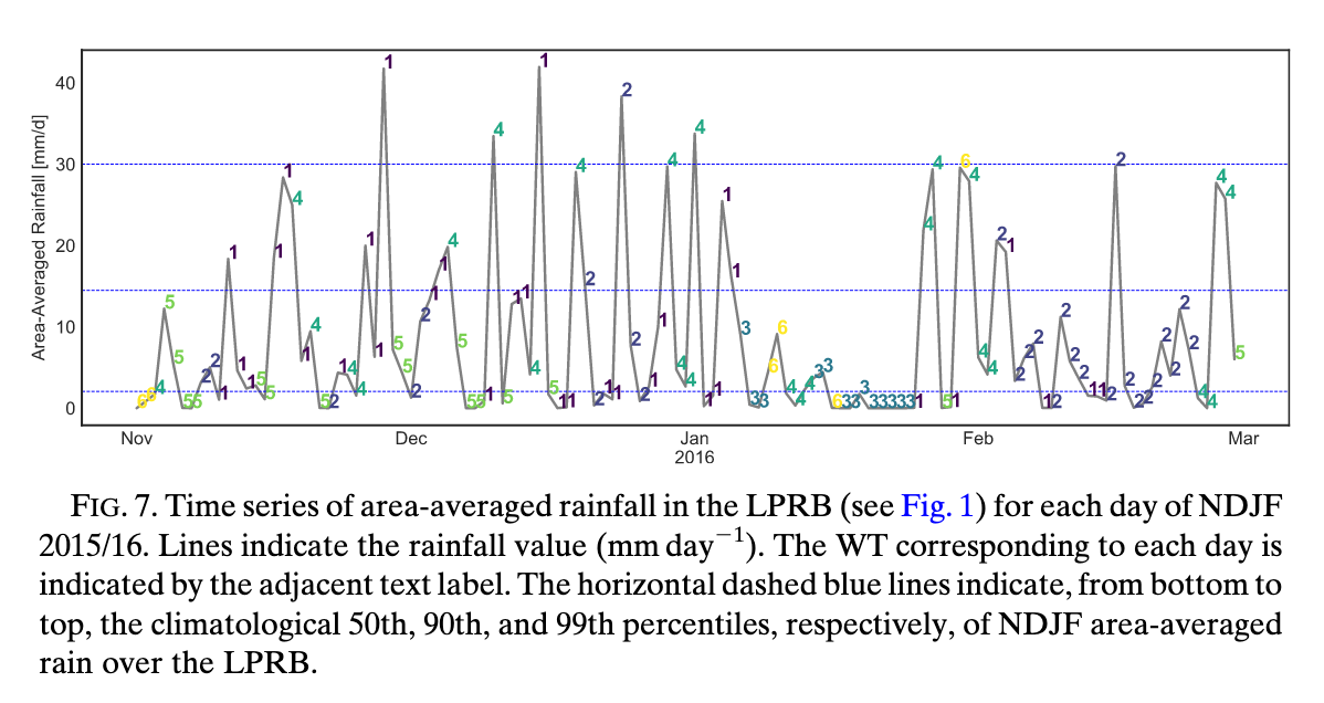
Q6: Looking at the colored bars in Fig. 7 for the 2015/16 summer, what do you notice about the frequency of different weather types? How does this explain the flood?
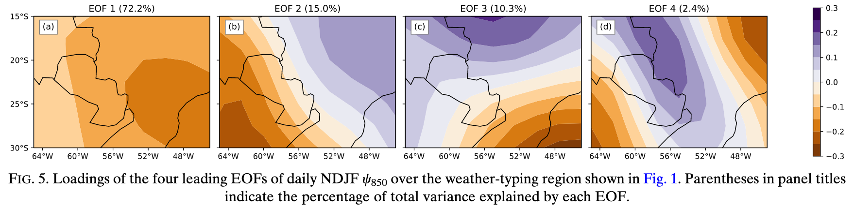
Q7: Before applying K-means clustering, the authors perform an EOF (PCA) analysis on the streamfunction anomaly field. Looking at Fig. 5, why did they do this EOF analysis rather than cluster the raw streamfunction maps directly?
Q10: \(K\)-means is a “hard” classification method. Looking at Fig. 7, what does this mean for any given day? What are the limitations of this approach, given that atmospheric flow is continuous and transitions smoothly from one state to another?
Q11: How does “forcing” days into discrete boxes affect the composite results shown in Fig. 6? Think about what happens when you include days that are “borderline” between two weather types.