Bias Correction and Downscaling
CEVE 543 - Fall 2025
- Motivation and GCM biases (minutes 0-4)
- Weather vs climate distinction + supervised learning (minutes 4-9)
- Delta method (minutes 9-21)
- QQ-mapping (minutes 21-33)
- Quantile delta mapping (QDM) (minutes 33-41)
- Uncertainty and critical considerations (minutes 41-44)
- Wrap-up and looking ahead (minutes 44-45)
1 Motivation: Why Bias Correction?
Minutes 0-4
- Climate models have systematic biases that directly affect impact assessments.
- Impacts depend on distributions (frequency, intensity, duration) — not just means or totals.
1.1 Two Types of GCM Biases
- Drizzle bias (pervasive):
- Too many light rainfall events with intensities too low relative to stations
- Root causes: spatial averaging within large grid cells (≈100–300 km) and sub-grid parameterizations
- Impacts: distorts frequency/intensity; affects crop growth, soil moisture dynamics, infiltration/runoff, and floods even when monthly totals match
- Dynamical biases (circulation errors):
- Examples: ENSO amplitude/frequency, monsoon onset/timing, midlatitude storm tracks
- Impacts: shifts climatology and interannual variability; affects predictability and teleconnections
Pick one impact domain (agriculture, floods, urban drainage, or energy). Which bias is more damaging in your domain—drizzle bias or dynamical bias—and why? What observable metrics would you compute to diagnose and quantify the bias?
Suggested format: 2 min pair + 2 min share.
1.2 Weather vs Climate
Minutes 4-9
- Weather forecasting: initial value problem with paired forecast–observation data → supervised learning works well.
- Climate projection: boundary value problem with no paired future observations → compare distributions under like-forcing; different statistical tools.
| Aspect | Weather forecasting | Climate projection |
|---|---|---|
| Mathematical framing | Initial value problem | Boundary value problem |
| Training data | Paired forecasts and observations | No pairs for the future; rely on historical distributions under same forcings |
| Typical methods | Supervised ML, data assimilation, super-resolution | Bias correction, quantile mapping, QDM, emulators respecting physics |
| Validation | Skill vs paired observations | Hindcast distributional match under historical forcings |
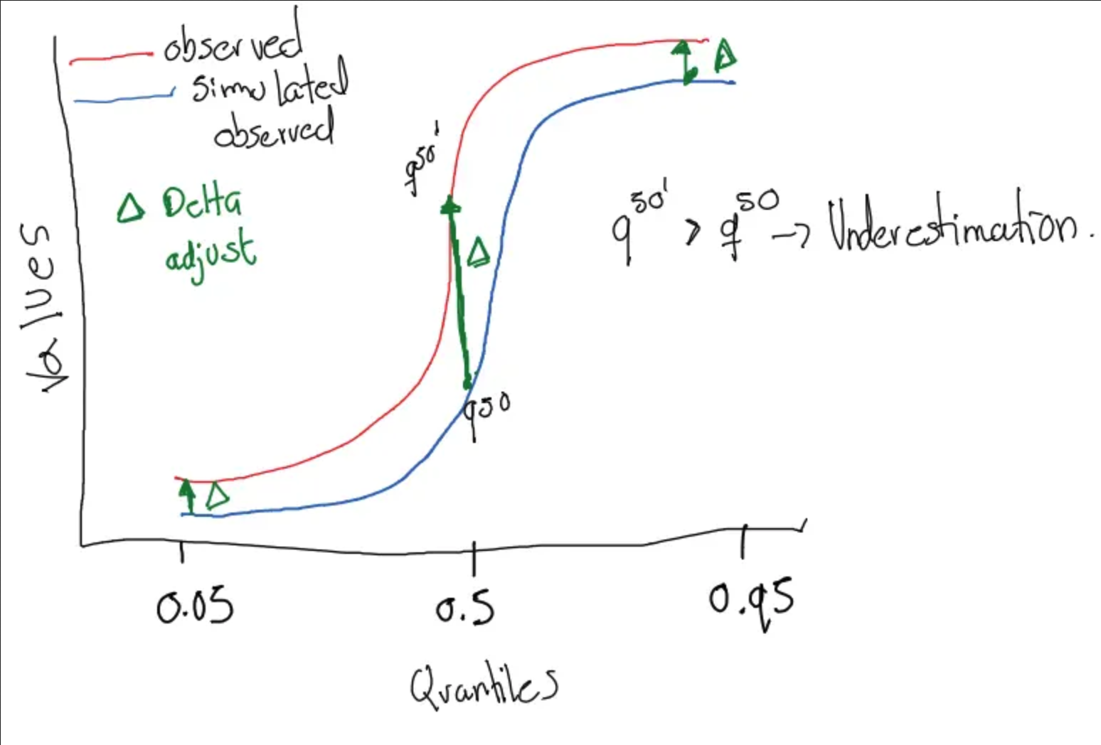
2 Delta Method
Minutes 9-21
The delta method is simple but widely used (Hay, Wilby, and Leavesley 2000).
2.0.1 Delta method (at a glance)
- Inputs: Observed historical series; GCM historical and future series (or statistics) by month/season
- Use when: You trust the modeled change signal more than model absolute levels
- Outputs: Corrected future series/statistics anchored to observations, preserving modeled change
- Pitfalls: Stationary-bias assumption; no frequency/intensity correction; deterministic
- Quick steps: compute Δ (additive for T, multiplicative for P) by month → apply Δ to observed baseline
2.1 Assumption and When to Use
- GCM can have systematic absolute biases (e.g., radiation/clouds, ocean heat transport, topography)
- Assume the modeled change signal (trend/delta) is credible
- Example: model is +2°C warm bias but simulates +3°C future warming → apply +3°C to observed baseline
2.2 Mathematical Framework
Notation:
- X^\text{obs}_\text{hist} = observed variable in historical period
- X^\text{GCM}_\text{hist} = GCM-simulated variable in historical period
- X^\text{GCM}_\text{fut} = GCM-simulated variable in future period
- \bar{X} = temporal average (e.g., monthly mean)
Compute the change (delta): \Delta = \bar{X}^\text{GCM}_\text{fut} - \bar{X}^\text{GCM}_\text{hist}
Apply to observations: X^\text{corr}_\text{fut} = X^\text{obs}_\text{hist} + \Delta
Note on notation: in the delta method, we apply the modeled change signal (the delta) to an observed baseline series. That’s why the baseline term is X^\text{obs}_\text{hist} (not GCM). By contrast, QQ-mapping and QDM directly transform the GCM daily values to corrected values.
2.3 Variants
For temperature, we typically use an additive delta: T^\text{corr}(d, m, y) = T^\text{obs}(d, m, y_\text{hist}) + [\bar{T}^\text{GCM}_\text{fut}(m) - \bar{T}^\text{GCM}_\text{hist}(m)]
Here d is the day of month, m is the calendar month, y is the year, and y_\text{hist} is a year from the historical period. We take a day from the historical record and add the monthly-mean temperature change.
For precipitation, we use a multiplicative delta: P^\text{corr}(d, m, y) = P^\text{obs}(d, m, y_\text{hist}) \times \frac{\bar{P}^\text{GCM}_\text{fut}(m)}{\bar{P}^\text{GCM}_\text{hist}(m)}
The same idea applies when the target is a derived statistic rather than the raw daily series.
2.4 Example Calculation
Suppose for July we have:
- Observed historical mean: \bar{T}^\text{obs}_\text{hist} = 25°\text{C}
- GCM historical mean: \bar{T}^\text{GCM}_\text{hist} = 27°\text{C} (2°C warm bias)
- GCM future mean: \bar{T}^\text{GCM}_\text{fut} = 30°\text{C}
The delta is \Delta = 30 - 27 = 3°\text{C}.
The corrected future temperature is T^\text{corr}_\text{fut} = 25 + 3 = 28°\text{C}.
We preserve the GCM’s 3°C warming signal while removing the 2°C warm bias.
2.5 Advantages and Limitations
- Advantages:
- Simple, transparent; preserves modeled change signal
- Works for many statistics (means, quantiles, variances)
- Seasonal specificity: apply deltas by month/season
- Limitations:
- Deterministic; no explicit uncertainty
- Assumes stationary bias structure across climate states
- Doesn’t correct frequency/intensity structure directly
3 Quantile-Quantile (QQ) Mapping
Minutes 21-33
QQ-mapping is more sophisticated and directly addresses the drizzle bias (Ines and Hansen 2006).
3.0.1 QQ-mapping (at a glance)
- Inputs: Daily/ sub-daily GCM and observed series (historical), by month/season
- Use when: Large-scale dynamics credible; need to fix wet-day frequency and intensity distribution
- Outputs: Bias-corrected series matching observed distribution (hist), applied to future with assumed stationarity
- Pitfalls: Can distort modeled change signal when applied to future; deterministic; tail extrapolation
- Quick steps: adjust wet-day frequency via threshold → map intensities via CDF-to-CDF transform (by month)
3.1 Assumption and When to Use
- Assumes large-scale dynamics are credible but frequency/intensity at sub-grid scales are biased
- Historical GCM–Obs distributional relationship is assumed to hold in the future
- Reasonable when GCM gets large-scale patterns right; risky if key processes are missing
The two figures below illustrate how QQ-mapping works:
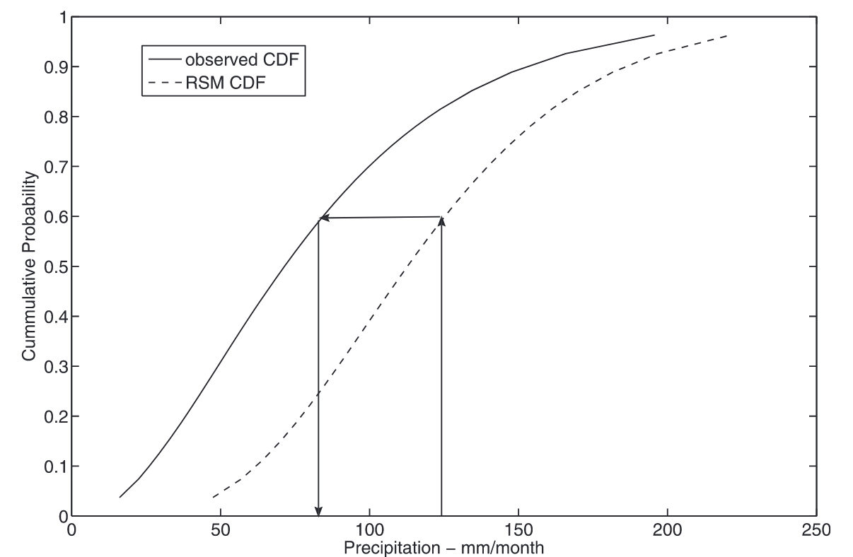
3.2 Two-Step Process
Notation:
- P^\text{GCM}(d, m, y) = daily GCM precipitation on day d of month m in year y
- P^\text{obs}(d, m, y) = daily observed precipitation
- F(\cdot) = cumulative distribution function (CDF)
- F^{-1}(\cdot) = inverse CDF (quantile function)
- \tilde{x} = threshold for defining “wet day” (typically 0.1 mm)
Step 1: Frequency correction
Find threshold \tilde{x}^\text{GCM} such that GCM wet-day frequency matches observed: F^\text{GCM}(\tilde{x}^\text{GCM}) = F^\text{obs}(\tilde{x}^\text{obs})
where \tilde{x}^\text{obs} = 0.1 mm is the observed wet-day threshold.
Invert to get: \tilde{x}^\text{GCM} = (F^\text{GCM})^{-1}\left(F^\text{obs}(\tilde{x}^\text{obs})\right)
Discard all GCM values below \tilde{x}^\text{GCM}. This removes excess drizzle events.
Step 2: Intensity correction
For each wet day i with x_i \geq \tilde{x}^\text{GCM}, map from GCM intensity distribution to observed: P^\text{corr}_i = (F^\text{obs}_I)^{-1}\left(F^\text{GCM}_I(P^\text{GCM}_i)\right)
where F^\text{GCM}_I is the CDF of GCM intensities above threshold \tilde{x}^\text{GCM} and F^\text{obs}_I is the CDF of observed intensities above threshold \tilde{x}^\text{obs}.
The intuition is to find where P^\text{GCM}_i falls in the GCM distribution, then sample the same percentile from the observed distribution.
3.3 Distribution Choices
For observed intensities (F^\text{obs}_I), we typically use a gamma distribution: f(x; \alpha, \beta) = \frac{1}{\beta^\alpha \Gamma(\alpha)} x^{\alpha-1} \exp\left(-\frac{x}{\beta}\right), \quad x > 0
The shape parameter \alpha is dimensionless and the scale parameter \beta has the same units as x. Both are estimated by maximum likelihood estimation (MLE).
For GCM intensities (F^\text{GCM}_I), two approaches are common. Gamma-Gamma (GG) fits a gamma distribution to both GCM and observed data. Empirical-Gamma (EG) uses the empirical CDF for GCM data but gamma for observed. Ines and Hansen (2006) found EG slightly better for their crop modeling application.
4 Quantile Delta Mapping (QDM)
Minutes 33-41
QDM blends the strengths of delta change and quantile mapping (Cannon, Sobie, and Murdock 2015). It corrects historical bias while preserving the GCM’s projected change at each quantile. This avoids “erasing” the modeled climate-change signal during bias correction.
4.1 Assumptions and Idea
- Historical quantile relation (model ↔︎ obs) is informative
- Modeled change signal by quantile is credible
- Procedure: quantile-map using historical relation → adjust by modeled change at the same percentile
4.2 Notation
- F^\text{mod}_\text{hist}, F^\text{obs}_\text{hist}: historical CDFs (model, observed)
- Q^\text{mod}_\text{hist}(p), Q^\text{mod}_\text{fut}(p), Q^\text{obs}_\text{hist}(p): corresponding quantile functions
- For a modeled future value y_i (from the GCM future series), define its modeled future percentile p_i = F^\text{mod}_\text{fut}(y_i)
4.3 QDM formula
Additive variables (e.g., temperature): x^{\text{QDM}}_{\text{fut}, i} = Q^\text{obs}_\text{hist}(p_i) + \Big[Q^\text{mod}_\text{fut}(p_i) - Q^\text{mod}_\text{hist}(p_i)\Big]
Multiplicative variables (e.g., precipitation): x^{\text{QDM}}_{\text{fut}, i} = Q^\text{obs}_\text{hist}(p_i) \times \frac{Q^\text{mod}_\text{fut}(p_i)}{Q^\text{mod}_\text{hist}(p_i)}
In other words, it’s just applying the delta method at each quantile after mapping to the observed distribution. Applying to intermediate percentiles typically requires an interpolation or similar (there are many flavors of these methods)
5 Critical Considerations
Minutes 41-45
5.1 Uncertainty
Bias correction is not a panacea and introduces additional uncertainty. Sources of uncertainty include:
- Sampling uncertainty (limited historical data). Recall: bias corrections are statistical models and are subject to the limitations of any statistical inference.
- Methodological details (distribution fits, thresholds)
- Model structural errors – different methods yield different results (see Lafferty and Sriver 2023)
5.2 Extrapolation
- All methods must extrapolate beyond calibration range
- QM: often uses constant (cap at max obs) or linear tail extrapolation → risk of unrealistic extremes or violations (e.g., negative P)
- Delta: assumes constant absolute (T) or relative (P) bias → may break if processes change (e.g., frontal → convective)
- No-analog futures: new circulation regimes, unprecedented T–q combos, shifts in precipitation mechanisms → transfer functions may fail
5.3 Missing Processes
You cannot correct for processes the GCM doesn’t simulate. Garbage in, garbage out still applies.
Consider tropical cyclones as an example. Many global GCMs don’t resolve tropical cyclones, which require roughly 50 km horizontal resolution. Observations clearly show TCs in coastal regions like Houston and Miami, but the GCM shows smooth, large-scale precipitation instead.
What happens with QQ-mapping? - It will create intense events to match the observed distribution, but: - Timing wrong (seasonally smeared vs clustered TC events) - Location wrong (tracks absent/shifted) - Dynamics wrong (no rotation/RI/structure)
5.4 Preparing for Wednesday
On Wednesday we will discuss Ines and Hansen (2006) in detail.
Key questions to consider while reading:
- How well does bias correction improve crop yield simulations?
- What limitations remain even after bias correction?
- Why are yields under-predicted even with “perfect” rainfall distributions?
The paper provides a concrete case study of the methods we discussed today and highlights remaining challenges.