Weather Typing and Synoptic Climatology
CEVE 543 - Fall 2025
- Weather typing: motivation and applications
- Clustering methods (K-means and alternatives)
- Dimension reduction via PCA
- Paper prep for Wednesday
1 Weather Typing and Analogs
1.1 The Power of Analogs
The fundamental problem:
Recall from 10/20 and 10/22 lectures:
- Climate models: systematic biases in local variables (drizzle bias, extremes)
- Coarse resolution: ~100-300 km gridcells
- “One gridcell = San Francisco to Sacramento”
- Too coarse for local impacts
Key insight: Models may get local precipitation wrong but large-scale patterns right!
The solution: Use analogs
Match large-scale patterns (models do well) to historical local impacts (what we observe).
Multiple analog methods:
- LOCA: Find matching historical days, select best analog per location (Pierce et al. 2015)
- Weather typing: Group states into discrete “types,” use conditional statistics (today’s focus)
- Archetype analysis: Identify extreme “corner” patterns (Steinschneider and Lall 2015)
- Self-organizing maps: Neural network preserving topology (Agel et al. 2018; Lima, AghaKouchak, and Lall 2017)
We’ll focus on weather typing, but the core idea generalizes.
1.2 Weather Typing Approach
Goal: Group similar atmospheric states into discrete “types”
Workflow:
- Identify recurring large-scale circulation patterns
- Link each weather type to observed local impacts
- When model simulates a weather type, apply local statistics
- Track weather type frequency changes under climate change
Applications:
- Statistical downscaling
- Bias correction conditioned on weather type
- Extreme event attribution
- Understanding circulation changes
Widely used in synoptic climatology and hydrology (Moron et al. 2015, 2008; Lee and Sheridan 2018; Rueda et al. 2016; Cagigal et al. 2020).
2 Clustering
2.1 Motivation
Goal: Partition observations into groups (clusters) with similar characteristics
Why cluster?
- Identify patterns in high-dimensional data
- Reduce continuous variability to discrete states
- Enable conditional statistics (e.g., P(rain | weather type))
2.2 K-means Clustering
Objective: Partition n observations into k clusters
Each observation is assigned to the cluster with the nearest mean (centroid).
Algorithm:
- Initialize k centroids randomly
- Assign each observation to the nearest centroid
- Uses a distance metric (typically Euclidean distance)
- Update the centroids by computing the mean of all assigned observations
- Repeat steps 2-3 until convergence (assignments no longer change)
Key choices:
Number of clusters k:
Use the “elbow method” to select k:
- Plot within-cluster sum of squares (WCSS) versus k
- WCSS measures total distance from points to their cluster centroids
- Look for an “elbow” where adding more clusters gives diminishing returns

Distance metric:
- Euclidean distance is most common
- Other options: Manhattan, cosine similarity
Initialization:
- Algorithm is sensitive to initial centroid placement
- Common practice: run multiple times with different initializations
- Keep the solution with lowest WCSS
Limitations:
- “Hard” classification (each point assigned to exactly one cluster)
- Assumes spherical clusters of similar size
- Sensitive to initialization
- Must specify k in advance
- Can struggle with outliers
- Sensitive to data scaling: K-means uses Euclidean distance, so variables with large variances will dominate the clustering. This motivates dimension reduction (PCA) before clustering. If you cluster on PCs, should you scale them to equal variance first? There’s no “right” or “wrong” answer - just be aware of the choice!
2.3 Alternatives
Gaussian Mixture Models (GMMs):
- Probabilistic approach
- Each point has probability of belonging to each cluster
- “Soft” classification
- More flexible than K-means
Self-Organizing Maps (SOMs):
- Neural network approach
- Maps high-D data to low-D grid
- Preserves topological structure
- Good for visualization
Hierarchical clustering:
- Builds tree of clusters (dendrogram)
- Agglomerative (bottom-up) or divisive (top-down)
- Don’t need to specify k in advance
- Can cut dendrogram at different levels
3 Dimension Reduction
Problem: Clustering algorithms work poorly in high dimensions
Why?
- Curse of dimensionality: points become equidistant
- Distance metrics become less meaningful
- More noise, slower computation
Solution: Reduce dimensionality first, then apply clustering
3.1 PCA
Also called: Empirical Orthogonal Functions (EOFs), Singular Value Decomposition (SVD)
Goal: Find orthogonal directions of maximum variance
3.1.1 Mathematical Setup
Data matrix: \mathbf{X} of size n \times p
- n = observations (e.g., time steps)
- p = variables (e.g., spatial locations)
- Each row = one observation
Objective: Find directions that maximize variance
3.1.2 First Principal Component
\mathbf{z}_1 = \mathbf{X} \boldsymbol{\phi}_1
- \boldsymbol{\phi}_1 = loading vector (size p \times 1)
- \|\boldsymbol{\phi}_1\|_2 = 1 (normalized)
- \mathbf{z}_1 = PC scores (size n \times 1)
For observation i: z_{i1} = \phi_{11} X_{i1} + \phi_{21} X_{i2} + \cdots + \phi_{p1} X_{ip}
Geometric interpretation: \boldsymbol{\phi}_1 is the direction of maximum variance

Subsequent PCs: \mathbf{z}_2, \mathbf{z}_3, \ldots
- Maximize the remaining (residual) variance after removing previous PCs
- Orthogonal to all previous PCs
- Each PC captures less variance than the previous one
3.1.3 Solution via Eigendecomposition
Step 1: Center the data \mathbf{X}_c = \mathbf{X} - \bar{\mathbf{X}}
Subtract column means so each variable has mean zero.
Step 2 (Optional): Standardize
Divide each column by its standard deviation.
Each variable then has unit variance.
This is a key decision:
- If you only center (Step 1), PCA is performed on the covariance matrix. Variables with higher variance will dominate the first PCs.
- If you standardize (Step 2), PCA is performed on the correlation matrix. All variables are treated as having equal variance. This is the right choice if your variables have different units.
Step 3: Compute the covariance matrix \mathbf{C} = \frac{1}{n-1} \mathbf{X}_c^T \mathbf{X}_c
This is a p \times p matrix.
Step 4: Solve the eigenvalue problem \mathbf{C} \boldsymbol{v}_j = \lambda_j \boldsymbol{v}_j
- \lambda_j = eigenvalue
- \boldsymbol{v}_j = eigenvector
Step 5: Sort the eigenvalues
Order them as: \lambda_1 \geq \lambda_2 \geq \cdots \geq \lambda_p
The corresponding eigenvectors are the loading vectors (principal components).
Step 6: Project the data \mathbf{Z} = \mathbf{X}_c \mathbf{\Phi}
- \mathbf{\Phi} = matrix of first k eigenvectors (size p \times k)
- \mathbf{Z} = PC scores (size n \times k)
3.1.4 Variance Explained
The eigenvalue \lambda_j equals the variance explained by PC j.
The fraction of total variance explained by the first k PCs is: \frac{\sum_{j=1}^k \lambda_j}{\sum_{j=1}^p \lambda_j}
Key assumption: Variance equals variability
This may not hold if:
- Data contain outliers
- Non-linear relationships are important
3.1.5 Climate Data Interpretation
Setup: Data matrix has time in rows, space in columns
Eigenvectors \boldsymbol{\phi}_j represent spatial patterns (EOFs)
Scores z_{ij} represent time series showing when each pattern is active
Reconstruction: \mathbf{X}_i \approx \sum_{j=1}^k z_{ij} \boldsymbol{\phi}_j^T
This reconstructs the data at time i using the first k EOFs.
3.1.6 Practical Considerations
Centering and anomalies:
Remove the time-mean at each location: x_{ij}' = x_{ij} - \bar{x}_j
For seasonal data, remove the seasonal climatology instead.
Standardization:
When should you standardize?
- Variables have different units → standardize
- Variables have similar units and scales → maybe not
- Standardization prevents one variable from dominating the PCA
Spatial weighting:
Latitude-longitude grids have unequal areas.
Grid cell area is proportional to \cos(\phi) where \phi is latitude.
Two approaches:
- Weight each data point by \sqrt{\cos(\phi)} before computing the covariance matrix
- This makes the covariance matrix effectively weighted by \cos(\phi) (since covariance involves products)
Why \sqrt{\cos(\phi)} and not \cos(\phi)?
The covariance matrix involves products of data values: X^T X.
If we weight data by \sqrt{\cos(\phi)}, the covariance becomes weighted by \cos(\phi).
This gives each unit area equal influence in the analysis.
Selecting the number of components:
Use a scree plot: plot variance explained versus component number.
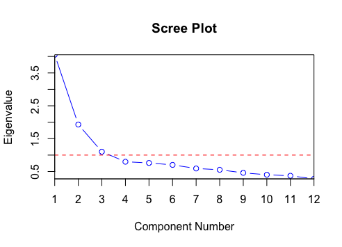
How to choose k?
There is no magical rule - it’s a trade-off between dimensionality and variance preserved.
Common approaches:
- Look for an “elbow” where additional components add little variance (subjective!)
- Choose k to explain a target fraction of variance (e.g., 80% or 90%)
- Rule of thumb (North et al. 1982): Check for separation in the eigenvalues. If eigenvalues are too “close” together, their corresponding EOFs may be mixed and not physically distinct.
- Consider the application: how much compression do you need?
- Try different values and see what works for your downstream task
Further Reading:
- SVD videos by Steven Brunton (watch Video 2)
- MIT PCA lecture
- James et al. (2013) Chapter 10.2
- NCAR EOF tutorial
4 Putting It All Together: The PCA-then-Cluster Pipeline
Typical workflow for weather typing:
- Start with high-dimensional data \mathbf{X} (size n \times p)
- Rows = time (days)
- Columns = space (grid cells) or other variables
- Perform PCA to get low-dimensional PC scores \mathbf{Z} (size n \times k)
- Each row is one day represented by k PC scores
- k \ll p (much fewer dimensions)
- (Optional but important) Scale the PC scores
- Should you scale PCs to equal variance before clustering?
- If yes: each PC weighted equally in clustering
- If no: PC1 (highest variance) dominates the clustering
- This is the choice made in Wednesday’s paper
- Run K-means clustering on the (possibly scaled) PC scores \mathbf{Z}
- Get k weather types
- Each day assigned to one weather type
Key decisions in this pipeline:
- How many PCs to retain? (Step 2)
- Should you scale the PCs before clustering? (Step 3)
- How many clusters k? (Step 4)
These choices are subjective but should be justified based on your scientific goals.
Preparing for Wednesday
Paper: Doss-Gollin et al. (2018)
Reading instructions:
- Read carefully: Sections 2-4, 6
- Skip: all of Section 5 (ENSO/MJO)
- Skip: ENSO/MJO discussion in Section 6
Discussion questions:
- Subjective choices (Section 3a):
- Why scale PCs to unit variance?
- Why choose K=6 clusters?
- How would K=8 change results?
- Hard vs. soft classification:
- K-means assigns each day to exactly one weather type
- What are limitations of “hard” classification?
- Atmospheric flow is continuous and can transition smoothly
- How does forcing into discrete “boxes” affect results?
- Bias correction application:
- You have a climate model that simulates 850-hPa streamfunction and precipitation
- How would you use the 6 weather types to bias correct precipitation?
- What biases would this method fix?
- What biases would it miss?